import quanguru as qg
import numpy as np
import matplotlib.pyplot as plt

9 - Simulation with a compute function

In previous tutorials, we covered the simulation of a single qubit, where we received a list of states from the runSimulation method, and used those states to compute some expectation values. In this tutorial, we will show an alternative that computes whatever we want during the evolution. The advantage in this approach is that we don’t have to keep a list of state vectors, which in general takes a lot memory. We, instead, only store some scaler quantities we are interested in.

Again, here, we will evolve a qubit under the unitary dynamics of its Hamiltonian with the initial state set to the equal superposition of and . We also set the total simulation time (with simTotalTime) and the step size (simStepSize).

# create the qubit and set its initial state and frequency
qub = qg.Qubit(frequency = 1)
qub.initialState = [0, 1]

# set the simulation time and step size
qub.simTotalTime = 2*np.pi
qub.simStepSize = 0.1

Now, we introduce the compute function and focus on its usage through QuantumSystem objects. We will cover more general usages of compute function/s in later tutorials, but the example here should suffice for most purposes.

We write compute function/s as generic functions, and store them in the compute attribute of QuantumSystem objects. During the time evolution of the system, the library calls the compute function/s at each time step of the evolution. When it is called in the background, the library passes the QuantumSystem object as the first argument of the compute function, and the state of the QuantumSystem at the current step of the evolution as the second argument.

Here, we will set a compute function to our Qubit, so the library will pass the qubit as the first argument, and its state at each time step as the second argument. Then, inside this function, we can compute anything we want from the state, and, below, we compute the expectation values of and operators. We still need to store these expectation values in somewhere, and this is where we use the .resultsDict attribute. We just call .resultsDict['someKey'].append(someValue) to store someValue with someKey, and the library takes care of the rest.

# create the operators for which we compute the expectation values
sigmaX = qg.sigmax()
sigmaZ = qg.sigmaz()

# write a compute function that takes two arguments: (i) a quantum-system (qsys) and (ii) a state
# compute whatever we want and store in .resultsDict
def compute(qsys, state):
    qsys.resultsDict['sigmax expectation'].append(qg.expectation(sigmaX, state))
    qsys.resultsDict['sigmaz expectation'].append(qg.expectation(sigmaZ, state))

# set the compute attribute of our qubit to compute function
qub.compute = compute

At this point, all the essential information are set, and we can run the simulation by qub.runSimulation(), which returns the list of states for the time evolution of our QuantumSystem.

But, in this case, we don’t want/need to store the states, because the compute function can and will compute all the quantities we are interested in. Therefore, we simply set simDelState to True, which will flag that we do not want to store the states.

qub.simDelStates = True
states = qub.runSimulation()

Now, we receive the results that we stored as qub.resultsDict['sigmax expectation']

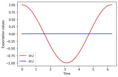
As expected, the expectation value of oscillates, while the expectation value of is constant (since )

plt.plot(qub.simulation.timeList, qub.resultsDict['sigmax expectation'], 'r-', label=r"$\langle \sigma_{x} \rangle$")
plt.plot(qub.simulation.timeList, qub.resultsDict['sigmaz expectation'], 'b-', label=r"$\langle \sigma_{z} \rangle$")

plt.legend()
plt.ylabel("Expectation values")
plt.xlabel("Time")

Text(0.5, 0, 'Time')

previous

8 - qRes attribute: an intro to Results objects

next

10 - Single parameter sweep