import quanguru as qg
import numpy as np
import matplotlib.pyplot as plt

14 - Time dependent Hamiltonian

In previous tutorials, the system Hamiltonians were time independent, and QuanGuru provides couple different methods to describe and simulate time-dependent Hamiltonians. In this tutorial, we demonstrate one (probably the most convenient and flexible) of these time-dependent Hamiltonian methods.

Here, we use the below single qubit Hamiltonian,

\(H=f_{z}J_{z} + f_{x}(t)\sigma_{x}\)

where the second term will be time dependent.

For the sake of the example, we won’t use the special Qubit class.

Define the system and parameters

We create a single qubit whose static Hamiltonian is set by \(J_{z}\) with frequency \(f_{z}=\texttt{qubFreq}\). Then we add a second term with operator \(\sigma_{x}\) and make its frequency time dependent.

The relevant information are:

• frequency: qubFreq for the static term and a time-dependent frequency for the drive

• operator: Jz for the qubit and sigma_x for the drive

• dimension: 2 for a qubit

We also compute useful derived quantities:

• \(\Omega_R = g\,A\) is the Rabi frequency set by coupling strength and drive amplitude

• \(\Delta = f_{z} - f_{\text{drive}}\) is the detuning

• \(\Omega = \sqrt{\Omega_R^2 + \Delta^2}\) is the generalized Rabi frequency

# define parameters
qubFreq = 1
driveFreq = 2
driveAmp = 1
drivePhase = 0
couplingStrength = 1

OmegaR = couplingStrength*driveAmp
detun = qubFreq-driveFreq
Omega = np.sqrt((OmegaR**2) + (detun**2))

We set the initial state to 1 (excited state for the qubit) and choose a total simulation time of one drive period with a small step size. We then provide a compute function that records the expectation value \(\langle\sigma_x\rangle\) at each time step.

# create the qubit and set its parameters
qub = qg.QuantumSystem(operator=qg.Jz)
qub.dimension = 2
qub.frequency = qubFreq

# add the drive term
secondTerm = qub.createTerm(operator=qg.sigmax)
secondTerm.frequency = driveFreq

# set the initial state
qub.initialState = 1

# set the simulation time and step size
qub.simTotalTime = 2*np.pi
qub.simStepSize = 0.01

# create the operators for which we compute the expectation values
sigmaX = qg.sigmax()

# write a compute function that takes two arguments: 1) a QuantumSystem (qsys) and 2) a state
# compute whatever we want and store in .resultsDict
# here we compute the expectation value of sigmaX and store it in 'sigmax expectation' resultsDict entry
def compute(qsys, state):
    qsys.resultsDict['sigmax expectation'].append(qg.expectation(sigmaX, state))

# set the compute attribute of our qubit to compute function
qub.compute = compute

C:\Users\Josh\Desktop\Masters Project\QuanGuru Code\QuanGuru\src\quanguru\classes\QSystem.py:353: UserWarning: QuantumSystem1 type (whether it is a single or composite system) is ambiguousIf it is intentional, please ignore this
  warnings.warn(f'{self.name} type (whether it is a single or composite system) is ambiguous'+\

Time-dependent term via a callback

We implement time dependence by assigning a function to the timeDependency attribute of the term. This function receives two arguments:

• st: the term (or system) whose attributes we will update

• ti: the current simulation time

Inside the function, we set st.frequency to a cosine modulation with drive frequency and phase:

\(f_{x}(t) = gA\cos(2\pi f_{\text{drive}}\,t + \phi)\)

This approach is flexible and can be applied to any QuantumSystem or Term object.

def secondTermTime(st, ti):
    st.frequency = couplingStrength*driveAmp*np.cos(2*np.pi*driveFreq*ti + drivePhase)

secondTerm.timeDependency = secondTermTime

At this point, all the essential information are set, and we can run the simulation by qub.runSimulation(), which returns the list of states for the time evolution of our QuantumSystem.

states = qub.runSimulation()

We verify that the number of propagator exponentiations equals the step count, which confirms the integrator advanced at the requested resolution.

# The number of exponentiations should be equal to the step count
print(qub._freeEvol.numberOfExponentiations, qub._freeEvol.numberOfExponentiations == qub.simulation.stepCount)

628 True

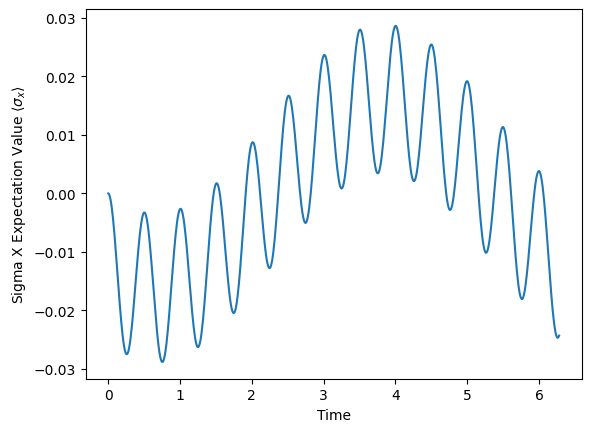
Finally, we plot \(\langle\sigma_x\rangle\) against time.

plt.plot(qub.simulation.timeList, qub.resultsDict['sigmax expectation'])
plt.xlabel('Time')
plt.ylabel(r'Sigma X Expectation Value $\langle\sigma_x\rangle$')

Text(0, 0.5, 'Sigma X Expectation Value $\\langle\\sigma_x\\rangle$')