import quanguru as qg
import numpy as np
import matplotlib.pyplot as plt

15 - Time dependent Hamiltonian 2

In previous tutorials, we covered how to set an initial state to a quantum system and how to describe its Hamiltonian.

Here, we will evolve the quantum system under the unitary dynamics of its Hamiltonian. First, we create a quantum system and describe its Hamiltonian

\(H=f_{z}J_{z} + f_{d}(t)\sigma_{+} + f_{d}^{*}(t)\sigma_{-}\)

where the second and third term will be time dependent.

Define the system and parameters

We create a single qubit whose static Hamiltonian is set by \(J_{z}\) with frequency \(f_{z}=\texttt{qubFreq}\). Then we add a second term with operator \(\sigma_{+}\) and third term with operator \(\sigma_{-}\) with time-dependent frequencies.

The relevant information are:

• frequency: qubFreq for the static term and a time-dependent frequency for the drive

• operator: Jz for the qubit, sigma_p and sigma_m for the drive

• dimension: 2 for a qubit

We also compute useful derived quantities:

• \(\Omega_R = g\,A\) is the Rabi frequency set by coupling strength and drive amplitude

• \(\Delta = f_{z} - f_{\text{drive}}\) is the detuning

• \(\Omega = \sqrt{\Omega_R^2 + \Delta^2}\) is the generalized Rabi frequency

# define parameters
qubFreq = 1
driveFreq = 2
driveAmp = 1
drivePhase = 0
couplingStrength = 1

OmegaR = couplingStrength*driveAmp
detun = qubFreq-driveFreq
Omega = np.sqrt((OmegaR**2) + (detun**2))

We set the initial state to 1 (excited state for the qubit) and choose a total simulation time of one drive period with a small step size. We then provide a compute function that records the expectation value \(\langle\sigma_x\rangle\) at each time step.

qub = qg.QuantumSystem(operator=qg.Jz)
qub.dimension = 2
qub.frequency = qubFreq

# add the drive terms
secondTerm = qub.createTerm(operator=qg.sigmap)
secondTerm.frequency = driveFreq

thirdTerm = qub.createTerm(operator=qg.sigmam)
thirdTerm.frequency = driveFreq

# set the initial state
qub.initialState = 1

# set the simulation time and step size
qub.simTotalTime = 2*np.pi
qub.simStepSize = 0.01

# create the operators for which we compute the expectation values
sigmaX = qg.sigmax()

# write a compute function that takes two arguments: (i) a quantum-system (qsys) and (ii) a state
# compute whatever we want and store in .resultsDict
def compute(qsys, state):
    qsys.resultsDict['sigmax expectation'].append(qg.expectation(sigmaX, state))

# set the compute attribute of our qubit to compute function
qub.compute = compute

Time-dependent terms via callbacks

We implement time dependence by assigning unique functions to the timeDependency attribute of each term. These functions receive two arguments:

• st: the term (or system) whose attributes we will update

• ti: the current simulation time

For the raising term \(\sigma_{+}\), we use a cosine modulation:

\(f_{+}(t) = gA\cos\big(2\pi f_{\text{drive}}\,t + \phi\big)\)

For the lowering term \(\sigma_{-}\), we use a complex exponential (negative-phase) modulation:

\(f_{-}(t) = -gAe^{-i\big(2\pi f_{\text{drive}}\,t + \phi\big)}\)

This approach is flexible and applies to any QuantumSystem or Term object.

# def secondTermTime(st, ti):
#     return -driveAmp*couplingStrength*np.exp(1j*(2*np.pi*driveFreq*ti + drivePhase))

def secondTermTime(st, ti):
    st.frequency = couplingStrength*driveAmp*np.cos(2*np.pi*driveFreq*ti + drivePhase)

def thirdTermTime(st, ti):
    st.frequency =  -driveAmp*couplingStrength*np.exp(-1j*(2*np.pi*driveFreq*ti + drivePhase))

secondTerm.timeDependency = secondTermTime
thirdTerm.timeDependency = thirdTermTime

At this point, all the essential information are set, and we can run the simulation by qub.runSimulation(), which returns the list of states for the time evolution of our QuantumSystem.

states = qub.runSimulation()

We verify that the number of propagator exponentiations equals the step count, which confirms the integrator advanced at the requested resolution.

# The number of exponentiations should be equal to the step count
print(qub._freeEvol.numberOfExponentiations, qub._freeEvol.numberOfExponentiations == qub.simulation.stepCount)

628 True

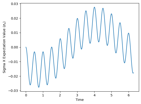
Finally, we plot \(\langle\sigma_x\rangle\) against time.

plt.plot(qub.simulation.timeList, qub.resultsDict['sigmax expectation'])
plt.xlabel('Time')
plt.ylabel(r'Sigma X Expectation Value $\langle\sigma_x\rangle$')

Text(0, 0.5, 'Sigma X Expectation Value $\\langle\\sigma_x\\rangle$')

Understanding Time-Dependent Hamiltonian Equivalence

This tutorial demonstrates a driven qubit system using two time-dependent terms with raising (\(\sigma_+\)) and lowering (\(\sigma_-\)) operators. Interestingly, this produces the same output as the simpler single-term approach in tutorial 14, which uses only \(\sigma_x\).

The Hamiltonians

Tutorial 14 (single drive term):

\[H_{T14} = f_z J_z + f_x(t)\sigma_x\]

where \(f_x(t) = gA\cos(2\pi f_{\text{drive}}t + \phi)\)

Tutorial 15 (two drive terms):

\[H_{T15} = f_z J_z + f_+(t)\sigma_+ + f_-(t)\sigma_-\]

where:

• \(f_+(t) = gA\cos(2\pi f_{\text{drive}}t + \phi)\) for the raising operator

• \(f_-(t) = -gAe^{-i(2\pi f_{\text{drive}}t + \phi)}\) for the lowering operator

Mathematical Equivalence

The key insight is the Pauli matrix identity:

\[\sigma_x = \sigma_+ + \sigma_-\]

Expanding the drive terms in Tutorial 15:

\[\begin{split}\begin{align} f_+(t)\sigma_+ + f_-(t)\sigma_- &= gA\cos(\omega t)\sigma_+ - gAe^{-i\omega t}\sigma_- \\ &= gA\frac{e^{i\omega t} + e^{-i\omega t}}{2}\sigma_+ - gAe^{-i\omega t}\sigma_- \end{align}\end{split}\]

where \(\omega = 2\pi f_{\text{drive}}t + \phi\).

After algebraic manipulation, the fast-rotating terms (at \(\pm 2\omega\)) average to zero, leaving:

\[f_+(t)\sigma_+ + f_-(t)\sigma_- \approx gA\cos(\omega t)(\sigma_+ + \sigma_-) = gA\cos(\omega t)\sigma_x\]

This exactly matches the drive term in Tutorial 14.