[1]:
import quanguru as qg
import numpy as np
16a - Jaynes-Cummings model of light-matter interaction#
Before demonstrating the Jaynes-Cummings (JC) Hamiltonian in QuanGuru, we provide some background for the JC Hamiltonian in this tutorial.
The JC Hamiltonian is commonly written as
\(H_{JC} = \hbar\omega_{c} a^{\dagger}a + \frac{1}{2}\hbar\omega_{q}\sigma_{z} + \hbar g(a^{\dagger}\sigma_{-} + a\sigma_{+})\)
where \(\sigma_{\pm} = (\sigma_{x} \pm i\sigma_{y})/2\) are raising/lowering operators for a two-level system, \(\sigma_{\mu}\) are the Pauli spin operators with \(\mu\in\{x,y,z\}\), \(a^{\dagger}\) and \(a\) are the creation and annihilation operators for the field mode, and \(\omega_{c}\), \(\omega_{q}\), and \(g\) are the cavity-field, qubit, and coupling (angular-) frequencies, respectively. Note that the above Hamiltonian is written in a common notation where the order of the sub-system Hilbert spaces is implicitly defined by the ordering in the coupling. This means, for example, that the composite form of the number operator is written explicitly as \((a^{\dagger}a)\otimes 1_{2,2}\) (similarly, \(a^{\dagger}\otimes\sigma_{-}\) and \(1_{d,d}\otimes\sigma_{z}\), where \(d\) is the truncation dimension for the cavity operators and \(\otimes\) is the tensor product).
Here, the eigenstates of the qubit are
Excited state : \(|e\rangle = \left[\begin{array}{ll} 1 \\ 0 \end{array}\right] \text{ (with eigenvalue }\frac{1}{2}\omega_{q})\)
Ground state: \(|g\rangle = \left[\begin{array}{ll} 0 \\ 1 \end{array}\right] \text{ (with eigenvalue }-\frac{1}{2}\omega_{q})\)
Together with the \(\sigma_{\pm} = (\sigma_{x} \pm i\sigma_{y})/2\) definition, we have
\(\sigma_{+} = \left[\begin{array}{ll} 0 & 1 \\ 0 & 0 \end{array}\right]\) so that \(\sigma_{+}|e\rangle = 0\) and \(\sigma_{+}|g\rangle = |e\rangle\)
\(\sigma_{-} = \left[\begin{array}{ll} 0 & 0 \\ 1 & 0 \end{array}\right]\) so that \(\sigma_{-}|e\rangle = |g\rangle\) and \(\sigma_{-}|g\rangle = 0\)
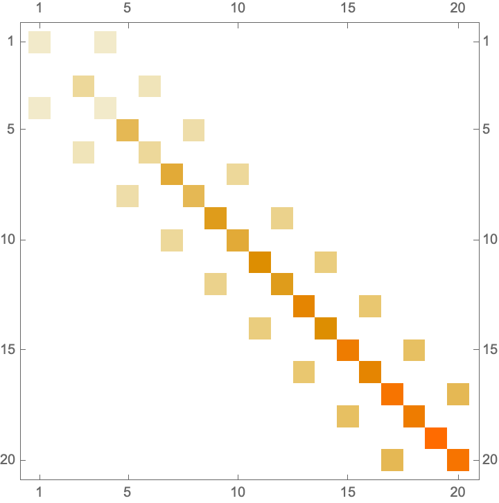
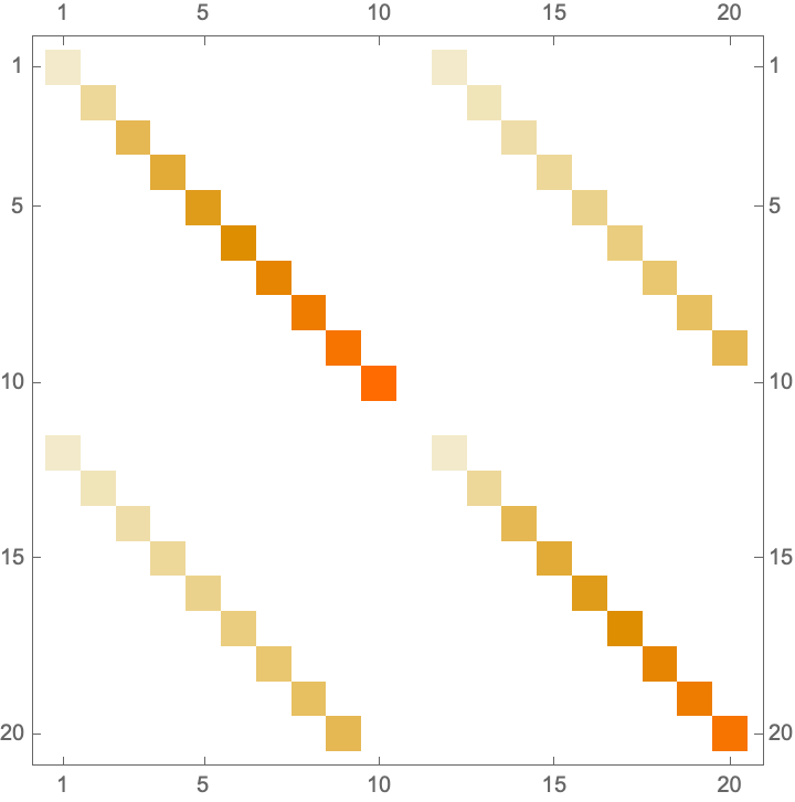
Finally, the matrix representations of JC Hamiltonian (with \(d=10\)) for two different cases of sub-system Hilbert space orders are
\(H_{JC} = \hbar\omega_{c} a^{\dagger}a\otimes 1_{2,2} + \frac{1}{2}\hbar\omega_{q}1_{d,d}\otimes\sigma_{z} + \hbar g(a^{\dagger}\otimes\sigma_{-} + a\otimes\sigma_{+})\)
\(H_{JC} = \hbar\omega_{c}1_{2,2} \otimes a^{\dagger}a + \frac{1}{2}\hbar\omega_{q}\sigma_{z}\otimes 1_{d,d} + \hbar g(\sigma_{-}\otimes a^{\dagger} + \sigma_{+}\otimes a)\)
In above convention, we see that the zero-excitation state \(|0, g\rangle\) (or, \(|g, 0\rangle\) in the qubit first order of sub-spaces) appears at \((2, 2)\) (or, at \((d+1, d+1)\) in the qubit first order of sub-spaces) index of the matrix representation. There are some other counter-intuitive details in above convention, and an alternative convention for JC Hamiltonian is to write the qubit term with a minus (\(- \frac{1}{2}\hbar\omega_{q}\sigma_{z}\)) so that the excited/ground state definition is switched
Excited state : \(|g\rangle = \left[\begin{array}{ll} 1 \\ 0 \end{array}\right] \text{ (with eigenvalue }-\frac{1}{2}\omega_{q})\)
Ground state: \(|e\rangle = \left[\begin{array}{ll} 0 \\ 1 \end{array}\right] \text{ (with eigenvalue }\frac{1}{2}\omega_{q})\)
However, in this alternative case, we also need to make some changes for the \(\sigma_{\pm}\) operators, otherwise, together with the \(\sigma_{\pm} = (\sigma_{x} \pm i\sigma_{y})/2\) definition, we have
\(\sigma_{+} = \left[\begin{array}{ll} 0 & 1 \\ 0 & 0 \end{array}\right]\) so that \(\sigma_{+}|g\rangle = 0\) and \(\sigma_{+}|e\rangle = |g\rangle\)
\(\sigma_{-} = \left[\begin{array}{ll} 0 & 0 \\ 1 & 0 \end{array}\right]\) so that \(\sigma_{-}|g\rangle = |e\rangle\) and \(\sigma_{-}|e\rangle = 0\)
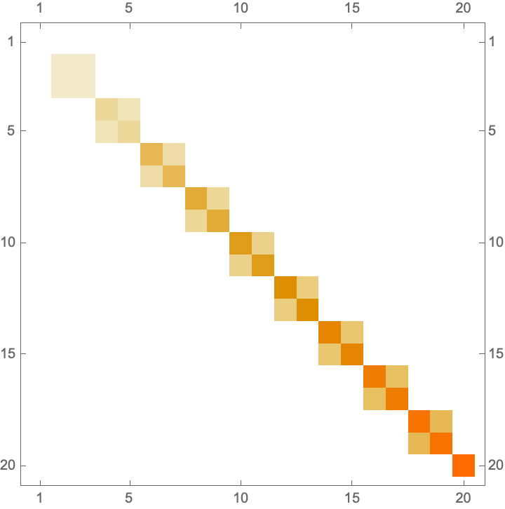
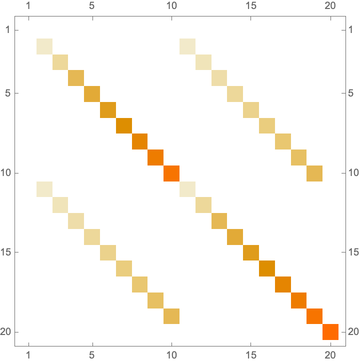
Here, we could introduce some unconventional definitions for \(\sigma_{\pm}\) by switching the \(\pm\) in their definition to \(\mp\), but we have a better alternative that is to replace \(\sigma_{-}\) and \(\sigma_{+}\) with 2-dimensional truncations of \(a\) and \(a^{\dagger}\), respectively. Then, the matrix representations of JC Hamiltonian (with \(d=10\)) for two different cases of sub-system Hilbert space orders are
\(H_{JC} = \hbar\omega_{c} a^{\dagger}a\otimes 1_{2,2} - \frac{1}{2}\hbar\omega_{q}1_{d,d}\otimes\sigma_{z} + \hbar g(a^{\dagger}\otimes a_{2,2} + a\otimes a_{2,2}^{\dagger})\)
\(H_{JC} = \hbar\omega_{c}1_{2,2} \otimes a^{\dagger}a + \frac{1}{2}\hbar\omega_{q}\sigma_{z}\otimes 1_{d,d} + \hbar g(a_{2,2}\otimes a^{\dagger} + a_{2,2}^{\dagger}\otimes a)\)
and, in the first case, we have \(|0, g\rangle\) at \((0, 0)\).