[1]:
import quanguru as qg
import numpy as np
import matplotlib.pyplot as plt
6 - Simulation of a Qubit with single term Hamiltonian#
In previous tutorials, we covered how to set an initial state to a quantum system and how to describe its Hamiltonian.
Here, we will evolve the quantum system under the unitary dynamics of its Hamiltonian. First, we create a quantum system and describe its Hamiltonian \(H=\frac{1}{2}f_{z}\sigma_{z} = f_{z}J_{z}\) and, for the sake of the example, we won’t use the special Qubit class.
[ ]:
qub = qg.QuantumSystem(operator=qg.Jz)
qub.dimension = 2
qub.frequency = 1
Now, let’s set its initial state to the equal superposition of \(|1\rangle\) and \(|0\rangle\).
[3]:
qub.initialState = [0, 1]
Finally, let’s set the total simulation time (with simTotalTime) and the step size (simStepSize), which is basically the sampling rate of the dynamics.
[4]:
qub.simTotalTime = 2*np.pi
qub.simStepSize = 0.1
At this point, all the essential information are set, and we can run the simulation by qub.runSimulation(), which returns the list of states for the time evolution of our QuantumSystem
[5]:
states = qub.runSimulation()
Given the time trace of states, we can calculate any quantity that we want, and, below, we calculate the expectation values of \(\sigma_{x}\) and \(\sigma_{z}\) operators.
[6]:
sigmaX = qg.sigmax()
sigmaZ = qg.sigmaz()
expectations = [[], []]
for st in states:
    expectations[0].append(qg.expectation(sigmaX, st))
    expectations[1].append(qg.expectation(sigmaZ, st))
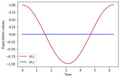
As expected, the expectation value of \(\sigma_{x}\) oscillates, while the expectation value of \(\sigma_{z}\) is constant (since \(\left[ H, \sigma_{z} \right] = 0\))
[7]:
plt.plot(qub.simulation.timeList, expectations[0], 'r-', label=r"$\langle \sigma_{x} \rangle$")
plt.plot(qub.simulation.timeList, expectations[1], 'b-', label=r"$\langle \sigma_{z} \rangle$")

plt.legend()
plt.ylabel("Expectation values")
plt.xlabel("Time")
[7]:
Text(0.5, 0, 'Time')